Multilevel Modeling and Effects Statistics for Sports Scientists in R
Why should sports scientist be familiar with mixed effects (multi-level) modeling and effect statistics…
Skill in analyzing longitudinal data is important for a number of practical reasons including; accounting for the dependencies created by repeated measures (athletes being measured over time), dealing with missing or unbalanced data (common occurrence in athlete monitoring practices), differentiating between-athlete from within-athlete variability, accounting for time-varying (e.g., workload, perceived fatigue) and time-invariant factors (e.g., gender, role, position) and establishing the influence of time (Windt et al. 2018). Multi-level models are very useful to a sports scientist because they can handle aforementioned complexities that are a natural part of player tracking/monitoring.
Measuring the magnitude or strength of the change of a health or performance outcome can also aid in the evaluation of the positive or negative consequences of an intervention or can be used to compare discrete groups/phases/conditions (e.g., male vs female, preseason vs. inseason, turf vs. grass surface). When assessing differences between said conditions, a common approach is using Cohen’s d, which is very similar to a standard difference score or z-score. Classic Cohen’s d requires the mean difference between conditions in the numerator and pooled standard deviation (i.e., combined standard deviation of each condition) in the denominator.
Cohen’s d Effect Size = (mean 1 – mean 2) ÷ between-athlete pooled SD
As mentioned, mixed models are unique becuase they can account for a number of variances (between-athlete/within-athlete, variability associated with time). However, this does present some issues when calculating classic cohen’s d directly from the model because Cohen’s d was developed for between-subjects research. With that in mind, the aim of this post is to set up a basic mixed model with player tracking (workload) data in R and explore the number of options one has to calculate effect statistics from the results.
Simulate Training Load Data
First things first, we need some player load data…which is not freely available but we can simulate a dataset to work with. With this data we are creating 20 athletes, with 50 sessions each (1000 total observations), assigning a mix of sessions by season phase (10 preseason, 30 inseason, 10 postseason), assigning each athlete a position, and randomly assigning a Total Distance value from a normal distribution with the mean equal to 5000 meters and a standard deviation of 1000 meters.
The problem with randomly assigning player distances from a normal distribution is that there will not be random variance in load by player, thus defeating the purpose of using mixed effects modeling. The random effect would be 0…so we need to introduce some variability. To do this, we can create an effect coefficient for each athlete and apply that to each individual player’s session load.
Also, we are going to look at differences between season phases so we need to introduce some variability in our independent variable. For the purposes of this example, we are going to assume that distances are ~1.2x higher on average during the preseason as compared to inseason or postseason phases.
library(tidyverse)
#set.seed for reproducibility
set.seed(415)

#simulate data
Athlete <- rep(paste('Athlete', 1:20), each = 50)
Session <- rep(1:50, times = 20)
Season <- rep(c("Preseason", "Inseason", "Postseason"), times = c(10, 30, 10))
Position <- rep(c("Point Guard", "Shooting Guard", "Small Forward", "Power Forward", "Center"), each = 50)
Distance <- rnorm(n = length(Athlete), mean = 5000, sd = 1000)


#create athlete effects
athleteeff = rnorm(20, 1, 0.1)
athleteeff_data <- data.frame(Athlete = paste('Athlete', 1:20), athleteeff)


#merge simulated data into a dataframe
data <- data.frame(Athlete, Session, Season, Position, Distance) %>%
  #increase preseason loads by 1.2x
  mutate(Distance = case_when(
    Season == "Preseason" ~ Distance*1.2,
    TRUE ~ Distance
  )
) %>%
  #join player effect coefficient
  left_join(athleteeff_data, "Athlete") %>%
  #multiply distances by each athletes effect coefficient
  mutate(Distance = Distance*athleteeff) %>%
  select(-athleteeff)
It’s always good to take a look at the structure of the data. Main thing is we want to make sure the data is in long format and each column is formatted appropriately (numeric, date, factor, etc.).
#structure of dataframe
str(data)
## 'data.frame':	1000 obs. of  5 variables:
##  $ Athlete : chr  "Athlete 1" "Athlete 1" "Athlete 1" "Athlete 1" ...
##  $ Session : int  1 2 3 4 5 6 7 8 9 10 ...
##  $ Season  : chr  "Preseason" "Preseason" "Preseason" "Preseason" ...
##  $ Position: chr  "Point Guard" "Point Guard" "Point Guard" "Point Guard" ...
##  $ Distance: num  6438 5325 10839 6508 8265 ...
#view dataframe
head(data)
##     Athlete Session    Season    Position  Distance
## 1 Athlete 1       1 Preseason Point Guard  6438.306
## 2 Athlete 1       2 Preseason Point Guard  5325.113
## 3 Athlete 1       3 Preseason Point Guard 10839.473
## 4 Athlete 1       4 Preseason Point Guard  6507.579
## 5 Athlete 1       5 Preseason Point Guard  8265.098
## 6 Athlete 1       6 Preseason Point Guard  6645.504
Fit Mixed Effects Model with lme4
With this model, we are doing a basic LMM, with Distance covered as our dependent variable, Season (preseason, inseason and postseason) as our independent variable (fixed effect) and we are clustering the data by athlete (random effect). Although one of the benefits of LMM is its abililtiy to incorporate multiple factors into a model (providing the ability to account for the variance of various contextual factors), for these purposes we’ll keep the model simple.
I always load the lmerTest package instead of lme4 by itself, doing so will load lme4 by default and the output will give you a p-value for each coefficient (which is typically needed in academia…not so much elsewhere).
library(lmerTest)

#fit model
fit <- lmer(Distance ~ Season + (1|Athlete), data = data)

#view results
summary(fit)
## Linear mixed model fit by REML. t-tests use Satterthwaite's method [
## lmerModLmerTest]
## Formula: Distance ~ Season + (1 | Athlete)
##    Data: data
##
## REML criterion at convergence: 16867.6
##
## Scaled residuals:
##     Min      1Q  Median      3Q     Max
## -3.4902 -0.5926 -0.0112  0.6361  4.1010
##
## Random effects:
##  Groups   Name        Variance Std.Dev.
##  Athlete  (Intercept)  336657   580.2
##  Residual             1217128  1103.2
## Number of obs: 1000, groups:  Athlete, 20
##
## Fixed effects:
##                  Estimate Std. Error      df t value Pr(>|t|)
## (Intercept)       5103.63     137.34   20.75  37.161   <2e-16 ***
## SeasonPostseason    36.71      90.08  978.00   0.408    0.684
## SeasonPreseason   1166.00      90.08  978.00  12.944   <2e-16 ***
## ---
## Signif. codes:  0 '***' 0.001 '**' 0.01 '*' 0.05 '.' 0.1 ' ' 1
##
## Correlation of Fixed Effects:
##             (Intr) SsnPst
## SeasnPstssn -0.164
## SeasonPrssn -0.164  0.250
We are given a few important metrics from the summary() function, such as the model estimates (coefficients) for each factor and also significant differences (to be explained). Fixed effects factor coefficients are listed in alphabetical order by default, so the Inseason phase (i.e. intercept) is listed first. If you want a particular factor as the intercept then you need to create an Ordered Factor (you can do this with the fct_relevel() function, which is available when you load the tidyverse package).
Even though we are working with a categorical independent variable it’s helpful to keep in mind that these models are linear regressions (lmer = Linear Mixed Effects Regression), so the first factor will always be the intercept. The significance of the first variable is always telling you if the intercept is significantly different from 0…it’s not telling you anything about its relationship with the other factors. Important things with this model summary are that the preseason is significantly different from inseason (at this point we don’t know if preseason loads are different from postseason loads). If we want to know where the differences are between factors, we need to run a post-hoc/follow-up statisical test such as Tukey HSD (which we will).
A More Detailed Summary…
I prefer to use the tab_model() function in the sjPlot package by Daniel Lüdecke to get a more detailed view of the model. You get a nice html table output that is publication worthy. There are several options to customize the table output, you can find that tutorial here. In addition to the standard components you get with a traditional summary() output, tab_model() provides a few other components we need to interpet the model such as the ICC value and marginal/conditional R^2^ values.
The higher the ICC value the more justified the use of LMM vs. a more traditional statistic (repeated measures ANOVA would be comparable in this instance). ICC’s can be interpeted as the proportion of variance explained by clustering. An ICC > 0.1 is generally accepted as the minimal threshold for justifying the use of LMM, so in other words at least 10% of the variance in Distance should be explained by clustering the observations by player.
# detailed summary
library(sjPlot)
tab_model(fit)
| Distance | |||
|---|---|---|---|
| Predictors | Estimates | CI | p |
| (Intercept) | 5103.63 | 4834.45 – 5372.80 | <0.001 |
| Season [Postseason] | 36.71 | -139.84 – 213.26 | 0.684 |
| Season [Preseason] | 1166.00 | 989.45 – 1342.55 | <0.001 |
| Random Effects | |||
| σ2 | 1217128.28 | ||
| τ00 Athlete | 336657.17 | ||
| ICC | 0.22 | ||
| N Athlete | 20 | ||
| Observations | 1000 | ||
| Marginal R2 / Conditional R2 | 0.121 / 0.312 | ||
In this instance, the ICC is 0.22 so the use of LMM is appropriate.
The other outputs of interest are our Marginal and Conditional R^2^ values (calculated based on Nakagawa et al.). These show the proportion of variance explained by the fixed effect only (Marginal R^2^) and fixed + random effect (Conditional R^2^), respectively.
So for this model, we would conclude that season phase is explaining ~12% of the distance covered in each session. It’s important to have this context becuase although there are significant differences in distance covered between the season phases, season phase by itself is not a strong determinant of session distance. On the other hand, the conditional R^2^ is ~0.31, so we can see that the proportion of variance explained by the combination of season phase and accounting for individual variance is much higher. When we sum the marginal R^2^ and the ICC value, we get a value quite close to our Conditional R^2^, this makes sense.
Visualize Model Effects
If you want to visualize the model (or any other mixed effects model [generalized, ordinal, etc.]), I would recommend using the ggeffects package (also by Daniel Lüdecke) combined with ggplot2 functions. You can find the ggeffects tutorial here. You can use the fit object with ggpredict() to create a data frame for plotting, pass a plot() function, and then add ggplot2() functions as needed to clean up the visualization. Here is a sample output from ggpredict().
library(ggeffects)
library(ggplot2)
#create plot dataframe
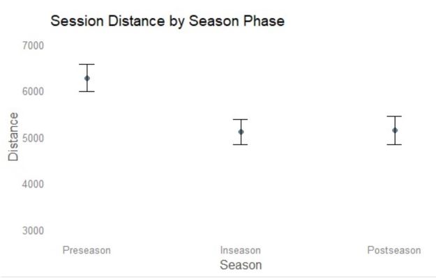
plot_data <- ggpredict(fit, terms = c("Season"))
plot_data
## # Predicted values of Distance
##
## Season     | Predicted |             95% CI
## -------------------------------------------
## Inseason   |   5103.63 | [4834.45, 5372.80]
## Postseason |   5140.34 | [4843.62, 5437.05]
## Preseason  |   6269.63 | [5972.91, 6566.34]
##
## Adjusted for:
## * Athlete = 0 (population-level)
Here is the plot output…
#create plot
plot_data %>%
  #reorder factor levels for plotting
  mutate(x = ordered(x, levels = c("Preseason", "Inseason", "Postseason"))) %>%
  #use plot function with ggpredict objects
  plot() +
  #add ggplot2 as needed
  theme_blank() + ylim(c(3000,7000)) + ggtitle("Session Distance by Season Phase")

Fit Tukey for Pairwise Comparisons
Since the model summary indicates we have some significant differences in session distance by season phase, the next step is to compare the levels against each other to see where the differences lie. We can tell by the model summary() output that Inseason and Postseason are significantly different than Preseason (model intercept), but we want to run this model through a post hoc test to confirm where the differences are.
library(multcomp)

# pairwise comparisons
fit_tukey <- glht(fit, linfct=mcp(Season="Tukey"))
summary(fit_tukey)
##
## 	 Simultaneous Tests for General Linear Hypotheses
##
## Multiple Comparisons of Means: Tukey Contrasts
##
##
## Fit: lmer(formula = Distance ~ Season + (1 | Athlete), data = data)
##
## Linear Hypotheses:
##                             Estimate Std. Error z value Pr(>|z|)
## Postseason - Inseason == 0     36.71      90.08   0.408    0.911
## Preseason - Inseason == 0    1166.00      90.08  12.944   <1e-05 ***
## Preseason - Postseason == 0  1129.29     110.32  10.236   <1e-05 ***
## ---
## Signif. codes:  0 '***' 0.001 '**' 0.01 '*' 0.05 '.' 0.1 ' ' 1
## (Adjusted p values reported -- single-step method)
As expected based on the model summary, both inseason and postseason session loads are less than the preseason. This makes sense. Preseason is used as a prepatory period and is accompanied by increased player loading.
Another important thing to note here, the difference estimates from this Tukey are the same as the lmer model summary, so we can also use these as our mean differences for the effect size calculations.
Calculating Effect Sizes
I’m not aware of any consensus on the best or preferred method of calculating effect sizes from within-subject designs. Jake Westfall goes into great detail here on the subject, detailing several of the ways cohens d and d-like effect sizes can be estimated. The important thing to note here is transparency when reporting a standardized effect size.
Option 1: Classical Cohen’s D Calculation
The effectsize() function in the effectsize package will give you classic Cohen’s d effect statistics from the lmer model output…
library(effectsize)

effectsize::effectsize(fit)
## # Standardization method: refit
##
## Parameter        | Coefficient (std.) |        95% CI
## -----------------------------------------------------
## (Intercept)      |              -0.18 | [-0.39, 0.02]
## SeasonPostseason |               0.03 | [-0.11, 0.16]
## SeasonPreseason  |               0.88 | [ 0.75, 1.02]
However, this output is somewhat limited, in that we are missing the Preseason - Postseason comparison effect statistic. The effectsize package supports lmerTest objects but unfortunatly will not work with our Tukey output. To get all comparison effect statistics using a traditional Cohen’s d, we can directly compare each variable.
To do that, we need to separate out the players distances by season phase.
preseason_data <- data %>% filter(Season == "Preseason") %>% dplyr::select(Distance)
inseason_data <- data %>% filter(Season == "Inseason") %>% dplyr::select(Distance)
postseason_data <- data %>% filter(Season == "Postseason") %>% dplyr::select(Distance)
There are several ways to do this. Firstly, you can write a cohen’s d function yourself. Credit to this post on StackOverflow. Note here that I’m not using the absolute value of the mean difference - as in the original cohen equation - this way we can see the direction of the effect.
cohens_d <- function(x, y) {
  lx <- length(x)- 1                  # Sample Size X
  ly <- length(y)- 1                  # Sample Size Y
  md  <- mean(x) - mean(y)            # Mean Difference
  csd <- lx * var(x) + ly * var(y)
  csd <- csd/(lx + ly)
  csd <- sqrt(csd)                    # Pooled SD

  md/csd                              # Cohen's d
}


cohens_d(inseason_data$Distance, preseason_data$Distance)
## [1] -0.9157833
…or there are R packages for computing classical cohen’s d such as lsr and effsize…please note that these functions take the absolute value of the mean difference so all results will be positive.
#install.packages("lsr")
#install.packages("effsize")
library(lsr)
lsr::cohensD(preseason_data$Distance, inseason_data$Distance)
## [1] 0.9157833
The effsize package has a cohen’s d function which will also give you 95%CI.
library(effsize)
effsize::cohen.d(preseason_data$Distance, inseason_data$Distance)
##
## Cohen's d
##
## d estimate: 0.9157833 (large)
## 95 percent confidence interval:
##     lower     upper
## 0.7493283 1.0822383
Given the options, let’s go ahead and use the cohen_d() function we wrote, create a dataframe and knit it into a table.
#gather cohen effect sizes
preseason_inseason_cohen <- cohens_d(preseason_data$Distance, inseason_data$Distance)
preseason_postseason_cohen <- cohens_d(preseason_data$Distance, postseason_data$Distance)
postseason_inseason_cohen <- cohens_d(postseason_data$Distance, inseason_data$Distance)


#make cohen dataframe
effect_data_cohen <- data.frame(
  "Season" = c("Preseason - Inseason", "Preseason - Postseason", "Postseason - Inseason"),
  "Effect Size Cohen" = c(preseason_inseason_cohen, preseason_postseason_cohen, postseason_inseason_cohen)) %>%
  rename(`Effect Size (Cohen)` = Effect.Size.Cohen) %>%
  mutate(`Effect Size (Cohen)` = round(`Effect Size (Cohen)`, 2))


knitr::kable(effect_data_cohen)
| Season | Effect Size (Cohen) |
|---|---|
| Preseason - Inseason | 0.92 |
| Preseason - Postseason | 0.88 |
| Postseason - Inseason | 0.03 |
Option 2: Standardized Effect Size using Residual Standard Deviation
This option is somewhat popular because the residual standard deviation is often assumed equivalent to the between-subjects standard deviation. However, that’s not always the case and is highly dependent on the data.
Extract Mean Differences
For the numerator we need mean differences, which we can grab from the Tukey summary (or you could gather them from the lmer model summary, results are the same…your choice).
#make tukey summary into an object
res <- summary(fit_tukey)

#extract first tukey comparison and make into an object
meandiff_1 <- res$test[-(1:2)]$coefficients[1]


#extract second tukey comparison and make into an object
meandiff_2 <- res$test[-(1:2)]$coefficients[2]


#extract third tukey comparison and make into an object
meandiff_3 <- res$test[-(1:2)]$coefficients[3]
One thing to consider when doing the extraction this way is that we are working Named Numbers, which you can see below when running the first coefficient.
res$test[-(1:2)]$coefficients[1]
## Postseason - Inseason
##              36.70945
If you want just the number, then you can use the unname() function.
unname(meandiff_1)
## [1] 36.70945
If you want the name of the object, use names().
names(meandiff_1)
## [1] "Postseason - Inseason"
We’ve already extracted mean differences for each comparison, so we only need to gather the residual standard deviation for this one. There are a few ways to do this, but the easiest is to call sigma from the model summary.
#extract the sd directly
summary(fit)$sigma
## [1] 1103.235
#create pooled residual sd object
pooled_sd_residual <- summary(fit)$sigma
#calculate effect sizes
effect_1_residual <- meandiff_1/pooled_sd_residual
effect_2_residual <- meandiff_2/pooled_sd_residual
effect_3_residual <- meandiff_3/pooled_sd_residual


#season column
Season <- c(names(meandiff_1), names(meandiff_2), names(meandiff_3))
#effects column
`Effect Size (Residual)` <- c(effect_1_residual, effect_2_residual, effect_3_residual)

#make residual effect dataframe
effect_data_residual <- as.data.frame(Season, `Effect Size (Residual)`) %>%
    mutate(`Effect Size (Residual)` = round(`Effect Size (Residual)`, 2))


#knit into table
knitr::kable(
  effect_data_residual
)
| Season | Effect Size (Residual) |
|---|---|
| Postseason - Inseason | 0.03 |
| Preseason - Inseason | 1.06 |
| Preseason - Postseason | 1.02 |
Option 3: Standardized Effect Size using All Variance Components
Probably the effect size calculation with the most academic support is taking the square root of the sum of all variance components in the model. This method was first discussed by Westfall, Judd, and Kenny (2014) and later included in a statisical tutorial of Effect Sizes and Power Analysis in Mixed Effects Models by Marc Brysbaert and Michaël Stevens (2018).
For this one we obviously need to gather all random effect variance components, which in this model are both the residual and within-athlete variances. You’ve already seen these in the model summary, so these calculations can be done simply by hand, but since we’re using R lets extract them using VarCorr().
#make VarCorr object from the model fit
vc <- VarCorr(fit)

#square root of the sum of model variance components (pooled standard deviation)
sqrt(as.data.frame(vc)$vcov[1] + as.data.frame(vc)$vcov[2])
## [1] 1246.509
#make pooled sd object
pooled_sd_allvar <- sqrt(as.data.frame(vc)$vcov[1] + as.data.frame(vc)$vcov[2])
#calculate effect sizes
effect_1_allvar <- meandiff_1/pooled_sd_allvar
effect_2_allvar <- meandiff_2/pooled_sd_allvar
effect_3_allvar <- meandiff_3/pooled_sd_allvar


#make All Variance effect column
`Effect Size (All Variance)` <- c(effect_1_allvar, effect_2_allvar, effect_3_allvar)


#make all variance dataframe
effect_data_allvar <-   as.data.frame(Season, `Effect Size (All Variance)`) %>%
    mutate(`Effect Size (All Variance)` = round(`Effect Size (All Variance)`, 2))


#knit into table
knitr::kable(
effect_data_allvar
)
| Season | Effect Size (All Variance) |
|---|---|
| Postseason - Inseason | 0.03 |
| Preseason - Inseason | 0.94 |
| Preseason - Postseason | 0.91 |
For comparison purposes, we can combine all three effect statistics into a single dataframe.
knitr::kable(
effect_data_cohen %>%
  left_join(effect_data_residual, by = "Season") %>%
  left_join(effect_data_allvar, by = "Season")
)
| Season | Effect Size (Cohen) | Effect Size (Residual) | Effect Size (All Variance) |
|---|---|---|---|
| Preseason - Inseason | 0.92 | 1.06 | 0.94 |
| Preseason - Postseason | 0.88 | 1.02 | 0.91 |
| Postseason - Inseason | 0.03 | 0.03 | 0.03 |
Add Effect Size Interpretations
Lastly, we can add interpretations to these effects. There have a been different propositions regarding the qualitative interpretation of ES’s. The original interpretation given by Cohen suggests <0.5 is a small effect, 0.5 to 0.7 is a moderate effect, and >0.8 is interpreted as a large effect. More recently Hopkins suggested a revised scale with threshold values at 0.2 (small), 0.6 (moderate), 1.2 (large), 2.0 (very large) and >4 (nearly perfect).
effect_interpretation <- effect_data_cohen %>%
   #interpret effect size
  mutate(`Hopkins Interpretation` = ifelse(abs(`Effect Size (Cohen)`) <= 0.2, "Trivial", ifelse(abs(`Effect Size (Cohen)`) <= 0.6, "Small", ifelse(abs(`Effect Size (Cohen)`) <= 1.2, "Moderate", ifelse(abs(`Effect Size (Cohen)`) <= 2, "Large", ifelse(abs(`Effect Size (Cohen)`) <= 4, "Very Large", "Nearly Perfect")))))) %>%
  mutate(`Cohen's Interpretation` = ifelse(abs(`Effect Size (Cohen)`) < 0.5, "Small", ifelse(abs(`Effect Size (Cohen)`) < 0.8, "Medium", "Large")))


knitr::kable(effect_interpretation)
| Season | Effect Size (Cohen) | Hopkins Interpretation | Cohen’s Interpretation |
|---|---|---|---|
| Preseason - Inseason | 0.92 | Moderate | Large |
| Preseason - Postseason | 0.88 | Moderate | Large |
| Postseason - Inseason | 0.03 | Trivial | Small |
As noted earlier and worth mentioning again, there are a number of ways to calculate standardized effect sizes and there really is not a universally accepted “right” way. Using residual SD and the square root of the sum of variance components from a mixed model for standardization are not traditional Cohen’s d statistics, so they should be referred to as standardized effect sizes. What we noticed from this dataset is that using the residual variance and all variance components in the denominator produced similar effect statistics becuase the within-athlete variability was quite small compared to the between-athlete variability. Both model effect statistic methods produced similar results than what we got by calculating cohen’s d directly from the data, again due to lower within-athlete variability. Although the effect statistics were similar in this simulated dataset, this will not always be the case, particularly when more complex models are used (e.g., multiple random intercepts, random slopes, or nested models) The important thing is to detail which method you are using and make sure to label it appropriately.
Dr. Ryan Curtis
Sports Science | Athletic Performance
Sports scientist/analyst, strength and conditioning coach, athletic trainer, researcher, author. Interested in all things related to optimizing performance and mitigating injury risk in sport.